The last half of the course was a writing period. Deadline for first draft of the essay was 25 January 2015, deadline for final version 30 January 2015. Submission is now closed, but used this easychair website.
Writing guidelines are available, and some suggestions for essay topics:
Writing guidelines are available, and some suggestions for essay topics:
Kernel Density Estimation
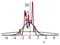
You are given a data set of samples from some distribution, and you want to visualize the data using a histogram. How wide should the bins of your histogram be?
As simple as it might seem, this question in fact does not have a single clear-cut answer. A distribution with lots of high and narrow spikes will be well represented by a histogram with narrow bins, but such a histogram will tend to mistake data sparsity for ruggedness in the density function when the samples come from a very flat distribution.
This problem is also found in the context of kernel density estimation, a technique that replaces the use of block-like bins with smooth functions such as lots of little Gaussian distributions stacked on top of each other. For such empirical density estimates, the variance of the little mini-distributions has to decrease as the number of data points increases, but the speed at which they must decrease will depend on the smoothness of the underlying distribution.
These issues raise a number of theoretical and practical problems: How would you choose, in practice, a good variance for the components of your density estimate? What kind of convergence guarantees can be given? Are there any diagnostics that can tell you when you have made your estimate too smooth or too jiggly? As a sanity check, you might want to try out any of your conclusions on this data set.
Some relatively recent textbooks that discuss these questions from a theoretical perspective are Larry Wasserman's All of Nonparameteric Statistics (2006, chs. 6.1–6.3) and Alexandre Tsybakov's Introduction to Nonparametric Estimation (2009, chapter 1.2). Numerous other texts and online resources exist too.
Randomization in Game-Theoretical Statistics
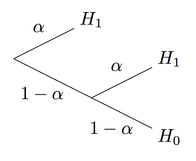
Suppose a coin with a bias of either .75 or .50. You flip the coin t = 5 times and record that it comes up heads k = 4 times. Which of the two hypotheses should you favor, a bias of .75 or a bias of .50?
Perhaps surprisingly, one reasonable answer to this question is “none of the above”: If we consider Nature as a malicious opponent who wants to spoil our attempts at prediction, we are in fact better off randomly selecting our guess than we are deterministically selecting the more likely candidate when k = 4.
The reason is that we might fear that Nature has selected a prior probability distribution which maximizes the error rate of our guessing strategy. Attempts to protect ourselves against such malicious environments have a strategic structure very similar to the game of matching pennies.
How does this idea play out in the general case, and in specific examples? Can you compute what the optimal policy is in the example above? How does this kind of strategic thinking compare to a Bayesian analysis? Does it provide a reasonable justification for the use of randomization in clinical trials, and can it perhaps be criticized for being overly pessimistic?
The game-theoretical formulation of statistical decision-making was most systematically pursured by Abraham Wald, who used it as a kind of justification for worst-case analysis. These ideas are explained in his book Statistical Decision Functions (1950) and in Girschick and Blackwell's Theory of Games and Statistical Decisions (1954), Ferguson's Mathematical Statistics (1967), and many other textbooks from that period.
The Dirichlet Process
A probability distribution can always be approximated by the empirical frequency distribution, but this approximation will be less accurate and more uncertain when the data set is small. There can therefore be some sense in relying on some reasonable initial guess and only gradually replace it with the empirical frequency distribution as more data comes in.
This is roughly the philosophy behind the Dirichlet Process, a family of probability distributions over probability distributions which extend the classical Bayesian approach to the estimation of the probability of a single event to a whole algebra of sets. Each of these probabilities are random variables, initially determined by a background measure, but gradually becoming more deterministic as more data comes in.
The Dirichlet process was first defined in the abstract by Thomas Ferguson (1973), but Sethuraman (1994) later provided a more intuitive interpretation in terms of countable lists of degenerate distributions. Since the Dirichlet Process has so many useful applications in machine learning, there are many introductory texts and tutorials, including this paper by Michael I. Jordan and this video lecture by Dilan Görür which discusses its use in practical clustering problems.
If you choose to write about this topic, you can either go in a more theoretical direction, explaining the connections between the various representations of the Dirichlet Process or its underpinnings in Kolmogorov's extension theorem, or in a more practical direction, building or describing a clustering method that can handle data sets such as this real-valued data set or this discrete one.
Stopping Rules and the Paradoxes of Statistical Testing
Biostatistician Jerome Cornfield writes (1966, p. 19):
“The following example will be recognized by statisticians with consulting experience as a simplified version of a very common situation. An experimenter, having made n observations in the expectation that they would permit the rejection of a particular hypothesis, at some predesignated significance level, say .05, finds that he has not quite attained this critical level. He still believes that the hypothesis is false and asks how many more observations would be required to have reasonable certainty of rejecting the hypothesis if the means observed after n observations are taken as the true values. He also makes it clear that had the original n observations permitted rejection he would simply have published his findings. Under these circumstances it is evident that there is no amount of additional observation, no matter how large, which would permit rejection at the .05 level. If the hypothesis being tested is true, there is a .05 chance of its having been rejected after the first round of observations. To this chance must be added the probability of rejecting after the second round, given failure to reject after the first, and this increases the total chance of erroneous rejection to above .05.”
Can this strange conclusion really be true? What is the philosophy underlying this “significance budget” interpretation, and why does it seem so counterintuitive?
The questions surrounding stopping rules and statistical tests have been central to the perennial debate between the frequentist and Bayesian approaches to statistics, and have been discussed by writers like Wald, Savage, Lindley, Stein, and others. Cornfield's paper gives a number of classic references, and David McKay discusses the issue from a Bayesian perspective in his textbook (ch. 37.2).
Bootstrapping (Sampling from a Sample)
Suppose you take a sample F' from a some distribution F and then estimate the mean m(F) by the sample average m(F'). How accurate is your estimate?
If you were able to draw a bunch of additional samples F' from F, you could use those to get a sense of how the sample average m(F') varies. However, you only have a single one. So how can you derive any conclusions about the distribution of m(F') from that?
One possible solution is to draw your ghost samples from the single sample you have rather than from the original distribution. Since the sample F' is itself a good approximation to F, a ghost sample F'' drawn from F' will also be a uniformly good picture F, although now with two layers of noise, like a photograph of a photograph. This idea is the basis of a technique known as bootstrapping. It is often used to construct confidence intervals or make various other kinds of inferences the distribution of empirical means, variances, or medians.
This something-for-nothing technique raises a number of questions about consistency, convergence rates, and asymptotic distributions that you can dig into. What happens, for instance, if you try to simulate the distribution of the sample average by bootstrapping from this sample from a Pareto distribution? What kind of theoretical results can you derive? In concrete cases, what kind of precision and confidence bounds do they permit you to compute? What are the monster cases that what cause them to fail?
There are a large number of introductions to the ideas behind bootstrapping and its properties. Brad Efron, one of its inventors, has written this accessible introduction to its philosophy as well as a number of other papers on the topic, and there are also book-length introductions such as Davison and Hinkley: Bootstrap Methods and Their Application (1997) and Mooney and Duval: Bootstrapping (1993).
The James-Stein Phenomenon
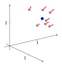
A planet is placed somewhere in three-dimensional space, and you want to estimate its position on the basis of a measurement X which is equal to the true position m plus some three-dimensional Gaussian noise with variance 1 in all directions. Given a single measured position X, what will be your best guess as to what the true position m of the planet is?
Up until the 1950s, any sane statistician would have said that the answer to this question would be m* = X. After all, guess at any other point in all of three-dimensional space would tend to bias the guess away from the actual data, and since this bias had no statistical justification, how could such a biased guess ever be better than an unbiased one?
This line of argument was shot down by the 1956 paper “Inadmissibility of the Usual Estimator for the Mean of a Multivariate Normal Distribution” by Charles Stein and its sequel by Stein and Willard James. James and Stein showed that one could get a uniformly better estimation performance by using estimate that was pulled slightly towards the origin of the space relative to the data point, thus trading off some data-sensitivity for robustness against noise. This trick is known as shrinkage as can be used in many different contexts.
How do such shrinkage estimators work? Why are they better than the obvious non-shrunk alternatives, intuitively and mathematically? How does one compute or estimate the optimal amount of contraction? How much improvement does it lead to, in theory and practice, for large and small data sets? How do estimators of this kind compare to optimal estimators? Why does this trick work in three dimensions but not in one or two? Can you think of other distributions where similar modifications of the obvious estimator would lead to better performance?
The James-Stein phenomenon is discussed in many textbooks on mathematical statistics, including Erich Lehmann's Theory of Point Estimation (1991, ch. 5), Richard Dudley's MIT course notes on mathematical statistics (online, ch. 2.7), and Larry Wasserman's All of Nonparametric Statistics (2006, ch. 7.6), and a entire book by Marvin Gruber is dedicated to the topic.
Support Vector Machines
The simplest way of building a binary classifier out of a labeled data set is simply to cut the space in two. Everything that falls on one side of the cut is then placed in one category, and everything that falls on the other side of the cut is placed in the other. This is an efficient and often good way of extracting information from a pattern, but it only has a very limited expressivity.
To increase the expressivity of the theory language, we can add more patterns to our portfolio besides simply straight cuts. But we can also, as first suggested by Valdimir Vapnik in the 1960s, map our low-dimensional data into a high-dimensional space and then perform our cut in the high-dimensional space in order to simulate a more expressive language. For instance, rather than dividing the two-dimensional space of (x,y)-coordinates into two halves, we could divide the three-dimensional space of (x^2,xy,y^2)-coordinates into two halves. Down in the two-dimensional space, this will simulate the effect of a non-linear curve.
This trick is the basis of the classification technique known as support vector machines, which is an example of a so-called kernel-based learning method. Common to many of these methods is the idea that the data set can be used as a basis for some high-dimensional space, so that decisions about new points in this space are made by literally decomposing the new into the old. This has computational advantages (it massively reduces the dimensionality) and conceptual (it allows for infinite-dimensional spaces).
There are numerous book-length treatments of support vector machines and related techniques, as well as course materials, video lectures and many other online materials. If you want to write about this topic, you can either approach it from a theoretical or practical perspective, but it would be a good idea to include at least some small-scale examples.
